matlab短期课程--应用
课程介绍
这仍是接着matlab短期课程的内容,但是更多的关注点在应用层面。
数值微积分
polynomial differentiation and integration
differentiation
- The derivative of a function \(f(x)\) is written as \[f'(x) \qquad \frac{df(x)}{dx}\]
- The rate of the change in the function \(f(x)\) with respect to x
- Geometrically,\(f'(x)\) represents the coefficient of the line tangent to the curve in the point \(x_0\)
polynomial differentiation
- Polynomials are often used in numerical calculations
- For a polynomial \[f(x)=a_nx^n+a_{n-1}x^{n-1}+ \dots a_1x+a_0\]
- The derivative is \[f'(x)=a_nnx^{n-1}+a_{n-1}(n-1)x^{n-2}+ \dots +a_1\]
Representing Polynomials in MATLAB
Polynomials were represented as row vectors
For example,consider the equation \[f(x)=x^3-2x-5\]
To enter this polynomial into MATLAB ,use
p=[1 0 -2 -5]一定要有常数项的数值
Values of Polynomials:ployval()
- polt the polynomial:\[9x^3-5x^2+3x+7 \] for \(-2 \le x \le 5\)
1 | a=[9,-5,3,7]; |
Polynomial Differentiation:polyder()
- Given \(f(x)=5x^4-2x^2+1\)
p=[5 0 -2 0 1]polyder(p)将求得\(f'(x)\)
- The value of \(f'(7)\)
polyval(polyder(p),7)
conv()可以对多项式进行乘法运算
polynomial integration
- For a polynomial \[f(x)=a_nx^n+a_{n-1}x^{n-1}+ \dots
a_1x+a_0\]
- The integration is \[\int f(x)dx=\frac{1}{n+1}a_nx^{n+1}+\frac{1}{n}a_{n-1}x^n+\dots+a_0x+k\] k值是需要提供给matlab的
Polynomial Integration:polyint()
- Given \[f(x)=5x^4-2x^2+1\]
P=[5 0 -2 0 1]polyint(P,3)需要给定最后的k值,这里的k是3
- The value of \(\int f(7) dx\)
polyval(polyint(P,3),7)
numerical differentiation and integration
numerical differentiation
- The simplest method: finite difference approximation
- Calculating a secant(割线) line in the vicinity of \(x_0\) \[f'(x_0)=\lim_{h\rightarrow
0}\frac{f(x_0+h)-f(x_0)}{h}\]
where \(h\) represents a small change in \(x\)
Differences:diff()
diff()calculates the differences between adjacent(临近的) elements of a vector
x=[1 2 5 2 1];diff(x);返回值内有4个Obtain the slope of a line between a points (1,5) and (2,7)
1
2
3
4
5
6
7
8>> x=[1 2];
>> y=[5,7];
>> slope=diff(y)./diff(x)
slope =
2
Numerical Differentiation Using diff()
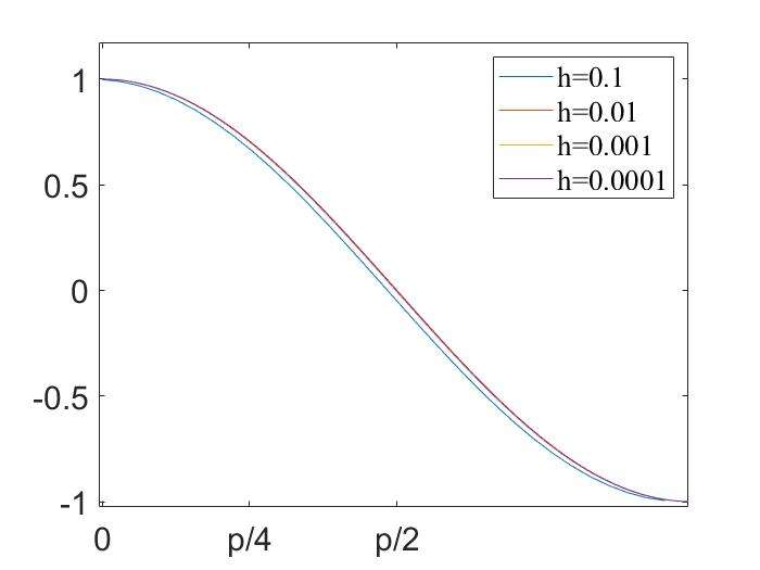
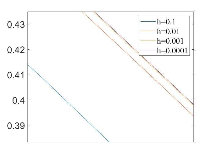
- Given \(f(x)=\sin(x)\),find \(f'(x_0) \qquad x_0=\pi/2\qquad\)using \(h=0.1\)
1 | x0=pi/2; |
How to Find the \(f'\) over An Interval \([0,2\pi]\)
- In the previous example,\(x_0=\pi/2\)
- Strategy:
- Create an array in the interval \([0,2\pi]\)
- The step is the \(h\)
- Calculate the \(f'\) at these points
- For example,
1
2
3
4clear;
h=0.5;x=0:h:2*pi;
y=sin(x);
m=diff(y)./diff(x)
Various Step Size
- The derivatives of \(f(x)=\sin(x)\) calculated using various \(h\) values
1 | g=colormap(lines);hold on; |
Exercise:
- Given\(f(x)=e^{-x}\sin(x^2)/2\),plot the approximate derivatives \(f'\) of \(h=0.1\quad 0.01 \quad 0.001\)
Second and Third Derivatives
- The second derivatives \(f''\) and third derivative \(f'''\) can be obtained using
similar approaches
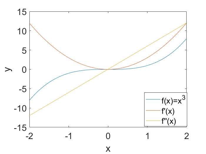
- Given \(f(x)=x^3\),plot \(f'\) and \(f' for -2 \le x \le 2\)
1 | x=-2:0.005:2; y=x.^3; |
numerical integration
- Calculating the numerical value of a definite integral \[s=\int_a^bf(x)dx \approx
\sum_{i=0}^nf(x_i)\int_a^bL_i(x)dx \]
- Quadrature(求积分) method approximating the integral by using a finite set of points
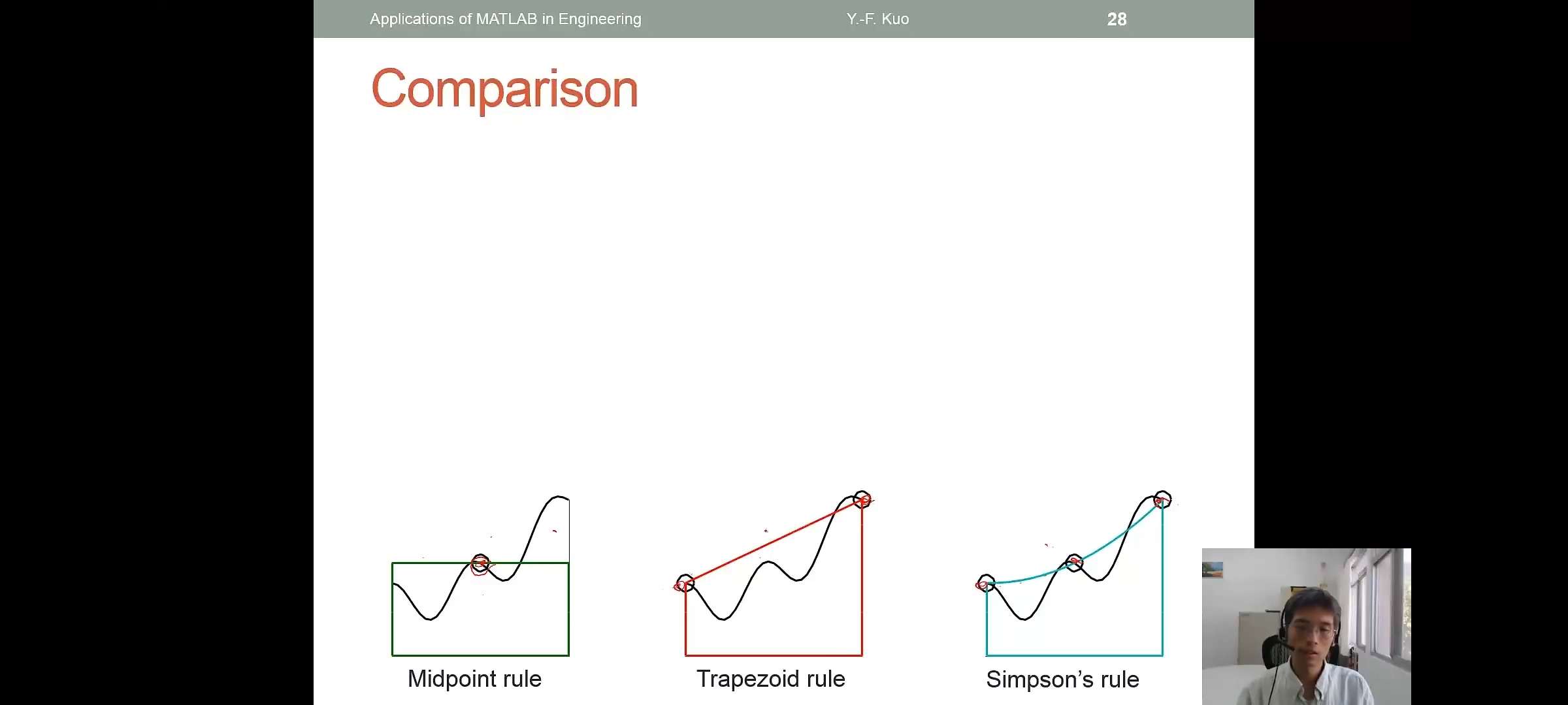
Numerical Quadrature Rules
- Basic quadrature rules
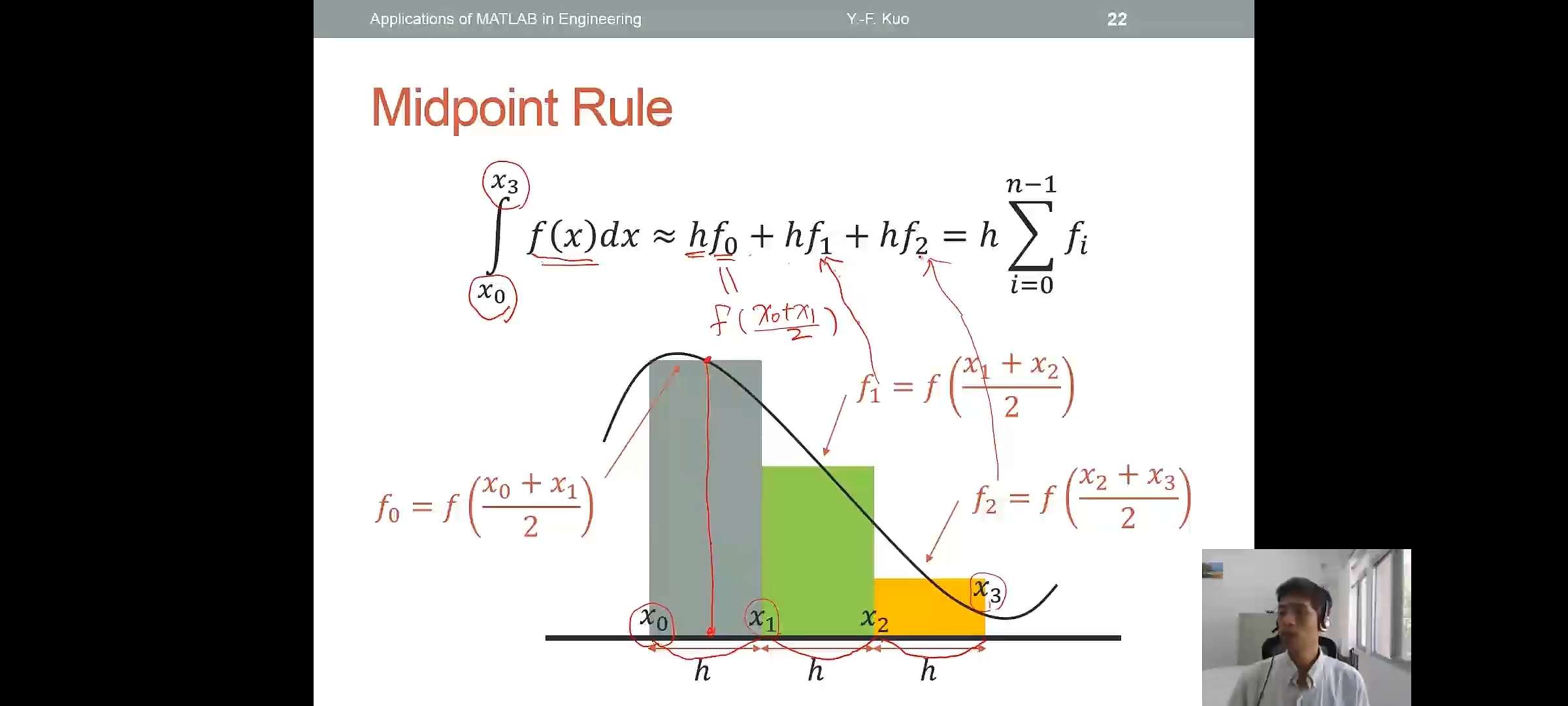
- Midpoint rule(zeroth-order approximation) 矩形预测
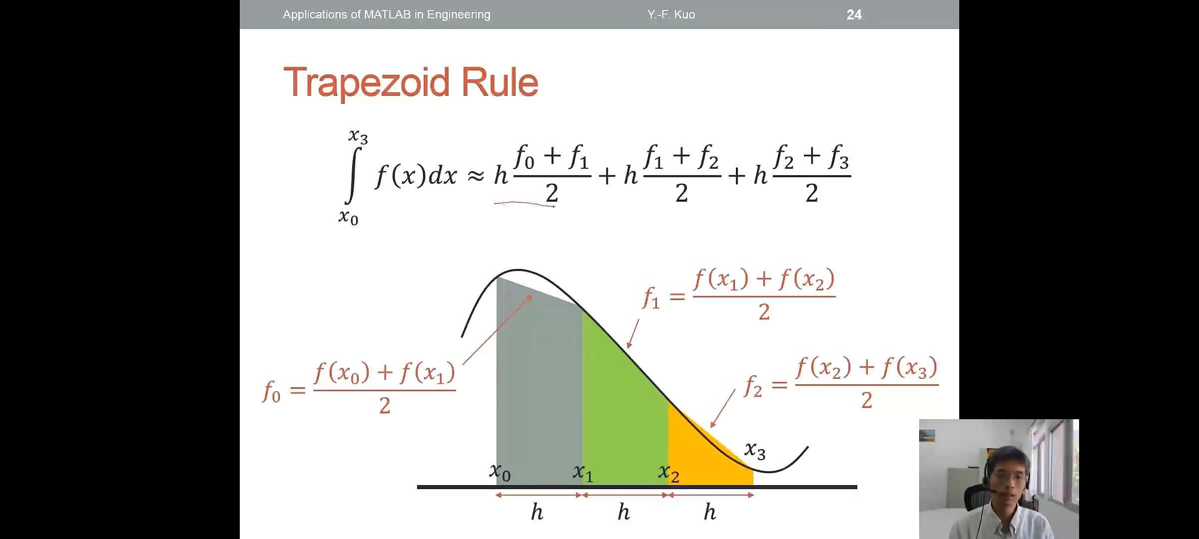
- Trapezoid rule(first-order approximation) 梯形预测
Midpoint Rule \[\int_{x_0}^{x_3}f(x)dx \approx hf_0+hf_1+hf_2=h\sum_{i=0}^{n-1}f_i\]
Midpoint Rule Using sum()
- Example \[A=\int_0^24x^3dx=16\]
1 | h=0.05; x=0:h:2; |
Trapezoid Rule
\[\int_{x_0}^{x_3}f(x)dx \approx h\frac{f_0+f_1}{2}+h\frac{f_1+f_2}{2}+h\frac{f_2+f_3}{2}\]
Trapezoid Rule Using trapz()
- Example \[A=\int_0^24x^3dx=16\]
- Alternative:
trapezoid=(y(1:end-1)+y(2:end))/2;
1 | h=0.05; x=0:h:2; |
Second-order Rule:\(\frac{1}{3}\)Simpson
\[\int_{x_0}^{x_2}f(x)dx \approx \frac{h}{3}(f_0+4f_1+f_2)\]
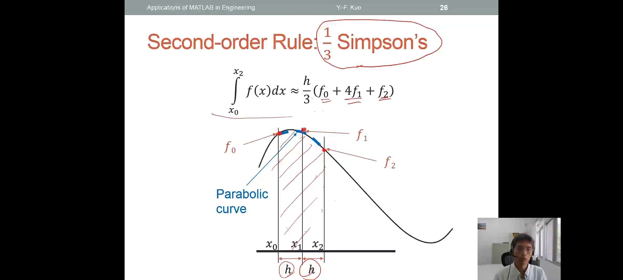 Simpson's Rule
- Example
\[A=\int_0^24x^3dx=16\]
1 | h=0.05; x=0:h:2; |
Comparison
Review of Function
Handles(@)
- A handle is a pointer to a function
- Can be used to pass functions to other functions 将函数传输给defined
function
- For example,the
input()of the following function is another function:1
2
3
4
5
6
7
8
9
10
11
12
13
14function [y]=xy_plot(intput,x)
y=input(x); plot(x,y,'r--');
xlabel('x'); ylabel('function(x)');
end
>> xy_plot(sin,0:0.01:2*pi)
错误使用 sin
输入参数的数目不足。
>> xy_plot(@sin,0:0.01:2*pi)%必须是@,告诉函数这是一个函数
ans =
列 1 至 11...
numerical
integration:integral()
- Numerical integration on a function from using global adaptive quadrature and default error tolerances
- Example
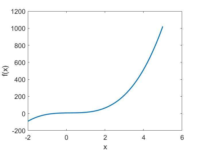
\[\int_0^2\frac{1}{x^3-2x-5}dx\]
1
2
3
4
5>> y=@(x) 1./(x.^3-2*x-5);
>> integral(y,0,2)%integral 第一个参数必须是matlab的函数,而非表达式
ans =
-0.4605
Double and Triple Integrals
- Example \[f(x,y)=\int_0^{\pi}\int_0^1(y \cdot \sin(x)+x\cdot cos(y))dxdy\]
- Example \[f(x,y,z)=\int_{-1}^{1}\int_0^{\pi}\int_0^1(y \cdot \sin(x)+z\cdot cos(y))dxdydz\]
1 | f=@(x,y) y.*sin(x)+x.*cos(y); |
方程式求根
Problem Statement
- Suppose you have a mathematical function \(f(x)\) and you want to find \(x_0\) such that \(f(x_0)=0\),e.g.\[f(x)=x^2-2x-8=0\]
- Solve the problem using MATLAB - Analytical Solutions(解析解) -
Graphical Illustration - Numerical Solutions(数值解)
symbolic approach
symbolic root finding approach
- performing mathematics on symbols,NOT numbers
- the symbols math are performed using "symbolic variables"(符号变量)
- use
symorsymsto create symbolic variables
- for example,
syms xx=sym('x')
symbolic root
finding:solve()
- Function
solvefinds roots for equations \[y=x \cdot \sin(x)-x=0 \] solve(equation,symbol)equation: \(y=0\) answer 也是symbol
Solving Multiple Equations
- Solve this equation using symbolic approach:
\[\begin{cases}
x-2y=5 \\
x+y=6 \\
\end{cases}
\]
1 | syms x y; |
Solving Equations Expressed in Symbols
- What if we are given a function expressed in symbols?
- \[ax^2-b=0\]
syms ax a bsolve(a*x^2-b)
- \(x\) is always the first choice to
be solved
- What if one wants th express \(b\) in terms of \(a\) and \(x\) ?
solve(a*x^2-b,b)将\(b\)设置为未知数
Exercise:
- Solve this equation for \(x\) using
symbolic approach \[(x-a)^2+(y-b)^2=r^2\]
- Find the matrix inverse using symbolic approach \[\begin{bmatrix} a&b \\ c&d\\ \end{bmatrix}\]
symbolic
differentiation:diff()
- Calculate the derivative of a symbolic function: \[y=4x^2\]
syms xy=4*x^5yprime=diff(y)
symbolic
integration:int()
- Calculate the integral of a symbolic function:\[z=\int ydx=\int x^2e^xdx,z(0)=0\]
syms xy=x^2*exp(x)z=int(y)z=z-subs(z,x,0)sub是substitution的缩写
1 | >> syms x |
Exercise:
\[\int_0^10\frac{x^2-x+1}{x+3}dx\]
Symbolic vs Numeric
| Advantages | Disadvantages | |
|---|---|---|
| Symbolic | 1.Analytical solutions 2.Lets you intuit things about solution form | 1. Sometimes can't be solved 2. Can be overly complicated |
| Numeric | 1. Always get a solution 2. Can make solutions 3. Easy to code | 1. Hard to extract a deeper understanding |
numeric root solvers
review of function handles(@)
- A handle is a pointer to a function
- Can be used to pass function to other functions
- For example,the
inputof the following function is another function:1
2
3
4
5
6function [y]=xy_plot(input,x)
y=input(x); plot(x,y,'r--');
xlabel('x'); ylabel('function(x)')
end
fsolve()
- A numeric root solver
- For example,solve this equation:\[f(x)=1.2x+0.3+sin(x)\]
f2=@(x)(1.2*x+0.3+x*sin(x));
fsolve(f2,0)f2 是 a function handle ,0 是initial guess
Exercise:
- Find the root for this equation:\[f(x,y)=\begin{cases} 2x-y-e^{-x} \\ -x+2y-e^{-y} \\ \end{cases}\] using initial value(初值)(x,y)=(-5,-5)
fzero()
- Another numeric root solver
- Find the zero if and only if the function cross the x-axis
f=@(x)x.^2fzero(f,0.1)结果显示无穷小 ,0.1附近的零点fsolve(f,0)结果显示为0- Options:
options=optimset('MaxIter',1e3,'TolFun',1e-10);1e3 is number of iterations 1e-10 is Tolerancefzero(f,0.1,options)
Finding Roots of Polynomials:roots()
- Find the roots of this polynomial: \[f(x)=x^5-3.5x^4+2.75x^3+2.125x^2-3.875x+1.25\]
roots([1 -3.5 2.75 2.125 -3.875 1.25])rootsonly works for polynomials,有时会得到复数解
How Do These Solvers Find the Roots?
- Now we are going to introduce more details of some numeric methods
Numeric Root Finding Methods
- Two major types:
- Bracketing methods (e.g.,bisection method) start with an interval that contains the root
- Open methods(e.g., Newton-Raphson method) start with one or more initial guess point
- Roots are found iteratively until some criteria are satisfied:
- Accuracy
- Number of iteration(迭代)
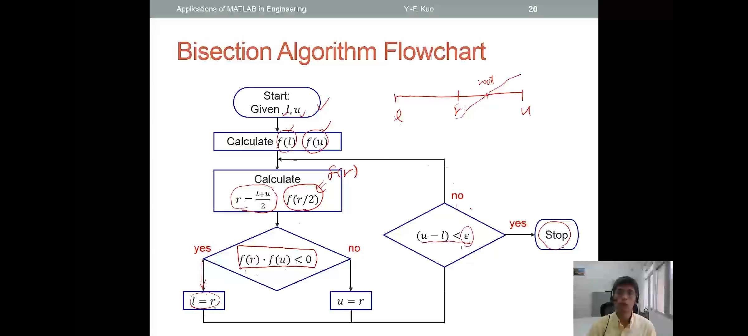
Bisection Method(Bracketing,二分法)
- Assumptions:
- \(f(x)\) contains on \([l,u]\)
- \(f(l) \cdot f(u) \lt 0\)
- Algorithm:
- \(r \rightarrow (l+u)/2\)
- if \(f(r) \cdot f(u) \lt 0\),then new interval \([r,u]\);if \(f(l) \cdot f(u) \lt 0\),then new interval \([l,r]\).
- Loop 2 End
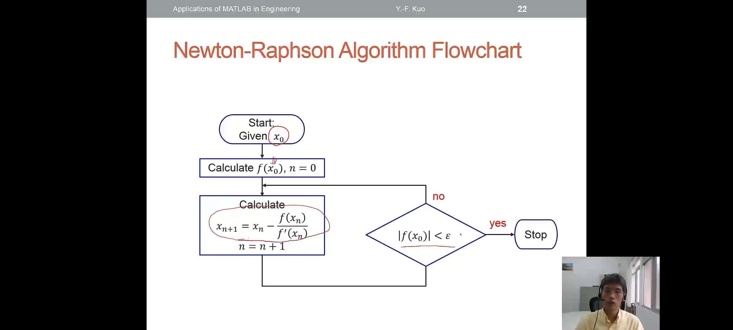
Newton-Raphson Method(Open)
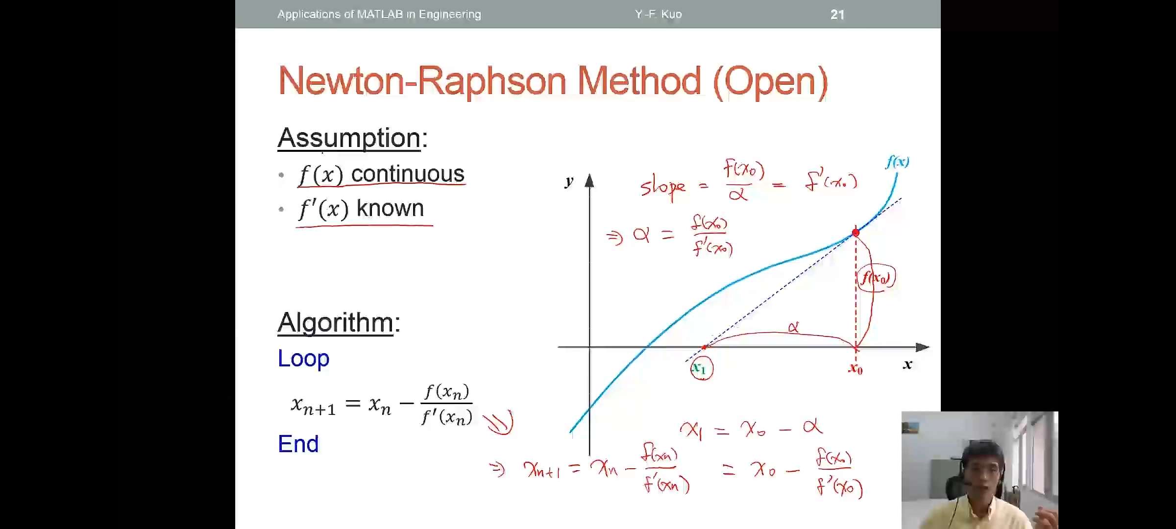
- Assumption:
- \(f(x)\) continuous
- \(f'(x)\) known
- Algorithm:
- Loop\[x_{n+1}=x_{n}-\frac{f(x_n)}{f'(x_n)}\]End
Bisection vs Newton-Raphson
- Bisection:
- Reliable
- No konwledge of derivative is need
- Slow
- One function evaluation per iteration
- Needs an interval \([a,b]\) containing the root \(f(a)\cdot f(b) \lt 0\)
- Netwon:
- Fast but may diverge
- Needs derivatives and an initial guess \(x_0\),f'(x_0) is nonzero
recursive function(递归函数)
- Function that call themselves
- Example,factorial of an integer \(n\) \[n!=1 \times 2 \times 3 \cdots \times n\]
- A factorial can be defined in terms of another factorial:\(n!=n \times (n-1)!\)
factorial recursive function
- The function includes a recursive cases and a base case
- The function stops when it reaches the base case
1
2
3
4
5
6
7function output = fact(n)
if n==1
output=1;% Base case
else
output =n*fact(n-1);%Recursive case
end
end
线性方程式与线性系统
linear equation
- Suppose you are given linear equation:\[\begin{cases}
3x-2y=5\\
x+4y=11 \\
\end{cases}\]
- Matrix notation:
\[\begin{bmatrix} 3 & -2 \\ 1 & 4 \\ \end{bmatrix} \cdot \begin{bmatrix} x \\ y \\ \end{bmatrix}= \begin{bmatrix} 5 \\ 11\\ \end{bmatrix}\]
对于矩阵的更多应用,可以参考D.Lay的《线性代数及其应用》
solving linear equations
- Successive elimination(through factorization)
- Cramer's method
Gaussian Elimination
Suppose given
\[\begin{cases} x+2y+z=2 \\ 2x+6y+z=7 \\ x+y+4z=3 \\ \end{cases}\]
\[ \Rightarrow \begin{bmatrix} 1& 2& 1& 2\\ 2& 6& 1& 7\\ 1& 1& 4& 3\\ \end{bmatrix}\]
通过高斯消元法最后可以得到:\[\begin{bmatrix} 1 & 2 & 1 & 2 \\ 0 & 2 & -1 & 3 \\ 0 & 0 & \frac{5}{2} & \frac{5}{2} \end{bmatrix}\]rref()
1 | A=[1 2 1;2 6 1;1 1 4]; |
LU Factorization
- Suppose we want to solve :\(Ax=b\),where \(A
\in \mathbb{R}^{m \times m}\)
- Decompose \(A\) into 2 triangular
matrices: \(A=L^{-1}U\)
- The problem become:\(Ax=b \Rightarrow \begin{cases} L^{-1}Ux=b\\ y=Ux \\ \end{cases}\)
- Strategies:
- Solve \(L^{-1}y=b\) to obtain \(y\)
- Then solve \(Ux=y\)
Lower and Upper Triangular Matrices
- Lower triangular matrix
\(L=\begin{bmatrix} 1 & 0 & 0 \\ \vdots & \ddots & 0 \\ \vdots & \cdots & 1 \\ \end{bmatrix} \in \mathbb{R}^{m \times m}\)
- Upper triangular matrix
\(U=\begin{bmatrix} \vdots & \cdots & \vdots \\ 0 & \ddots & \vdots \\ 0 & 0 & \vdots \\ \end{bmatrix} \in \mathbb{R}^{m \times m}\)
How to obtain \(L\) and \(U\)?
- The matrices \(L\) and \(U\) are obtained by using a serious of
left-multiplication ,i.e.,\[L_m\cdots L_2
L_1A=U\]
- Example,
\[A=\begin{bmatrix} 1&1&1 \\ 2 & 3 & 5 \\ 4&6&8\\ \end{bmatrix}\] \[L_1A=\begin{bmatrix} 1 & 0& 0 \\ -2 &1 &0 \\ -4 &0&1 \\ \end{bmatrix} \cdot \begin{bmatrix} 1 &1 &1\\ 2 &3 &5\\ 4 &6 &8\\ \end{bmatrix}= \begin{bmatrix} 1 &1 &1\\ 0 &1 &3\\ 0 &2 &4\\ \end{bmatrix}\]
\[L_2(L_1A)=\begin{bmatrix} 1&0 &0\\ 0 &1 &0\\ 0 &-2 &1\\ \end{bmatrix} \cdot \begin{bmatrix} 1 &1 &1\\ 0 &1 &3\\ 0 &2 &4\\ \end{bmatrix}= \begin{bmatrix} 1 &1 &1\\ 0 &1 &3\\ 0 &0 &-2\\ \end{bmatrix}=U\]
- 分解的目标在于最后化为三角型矩阵。故可以预先确定一些矩阵相应位置上的元素,然后再来解出其他位置上的元素
LU Factorization lu()
[L,U,P]=lu(A);
- Solving:\(\begin{cases} L^{-1}y=b \\ Ux=y
\\ \end{cases}\)
inv(L) U
Matrix Left
Division:\ormldivide()
- Solving systems of linear equations \(Ax=b\) using factorization methods:
\[ \begin{cases} x+2y+z=2\\ 2x+6y+z=7\\ x+y+4z=3\\ \end{cases}\]
A=[1 2 1;2 6 1;1 1 4]; b=[2;7;3];
x=A\b
Matrix Decomposition Functions
| code | 解释 |
|---|---|
qr |
Othogonal-triangular decomposition |
ldl |
Block LDL'factorization for Hermitian indefinite matrices |
ilu |
Sparse incomplete LU factorization |
lu |
LU matrix factorization |
chol |
Cholesky factorization |
gsvd |
Generalized singular value decomposition |
svd |
Singular value decomposition |
Cramer's(Inverse) Method
Given the problem \[\begin{bmatrix} 3 & -2 \\ 1 & 4 \\ \end{bmatrix} \cdot \begin{bmatrix} x \\ y \\ \end{bmatrix}= \begin{bmatrix} 5 \\ 11\\ \end{bmatrix}\]
Suppose there exists the \(A^{-1} \in \mathbb{R}^{m \times m}\) such that\[AA^{-1}=A^{-1}A=I\]
The variable \(x\) is:\(x=A^{-1}b\)
Inverse Matrix
- For a matrix, the inverse is defined as: \[A^{-1}=\begin{bmatrix}
a&b\\
c&d\\
\end{bmatrix}^{-1}=
\frac{1}{det(A)}adj(A)=
\frac{1}{det(A)}
\begin{bmatrix}
d&-b \\
-c&a\\
\end{bmatrix}\] where \(det(A)\)
is the determinant:\[det(A)=|ad-bc|\]
- Properties:\(A=(A^{-1})^{-1}\),\((kA)^{-1}=k^{-1}A^{-1}\)
Solving Equation Using Cramer's Method
- \(x=A^{-1}b\)
x=inv(A)*b - The inverse matrix does not
exist,
det(A)若等于零,则该矩阵的逆是不存在的
Exercise:
- Plot the planes in 3D:\(\begin{cases} x+y+z=0\\ x-y+z=0\\ x+3z=0\\ \end{cases}\)
Problem with Cramer's Method
- Recall that \(A^{-1}=\begin{bmatrix} a&b\\ c&d\\ \end{bmatrix}^{-1}= \frac{1}{det(A)}adj(A)\)
- The determinant is zero if the equations are singular ,i.e.,\(det(A)=0\)
- The accuracy is low when the determinant is very close to zero ,i.e.,\(det(A)\backsim 0\)
Functions to Check Matrix Condition
| code | 解释 |
|---|---|
cond |
Matrix condition number |
rank |
Matrix rank |
- Check the change in \(x\) if \(A\) changes by a "small" amount \(\delta A\): \[\frac{||\delta A||}{||x||} \le k(A)\frac{||\delta A||}{||A||}\], where \(k(A)\) is the condition number of \(A\)
- A small \(k(A)\) indicates a
well-conditioned matrix
cond(A)
linear system
Suppose you are given linear equations:\[\begin{cases} 2 \cdot 2 - 12 \cdot 4=x\\ 1 \cdot 2 - 5\cdot 4 =y\\ \end{cases}\]
Matrix notation:
\[\begin{bmatrix} 2&-12\\ 1&-5\\ \end{bmatrix} \cdot \begin{bmatrix} 2\\ 4\\ \end{bmatrix} = \begin{bmatrix} x\\ y\\ \end{bmatrix}\]Note that the differences between linear system and linear equation
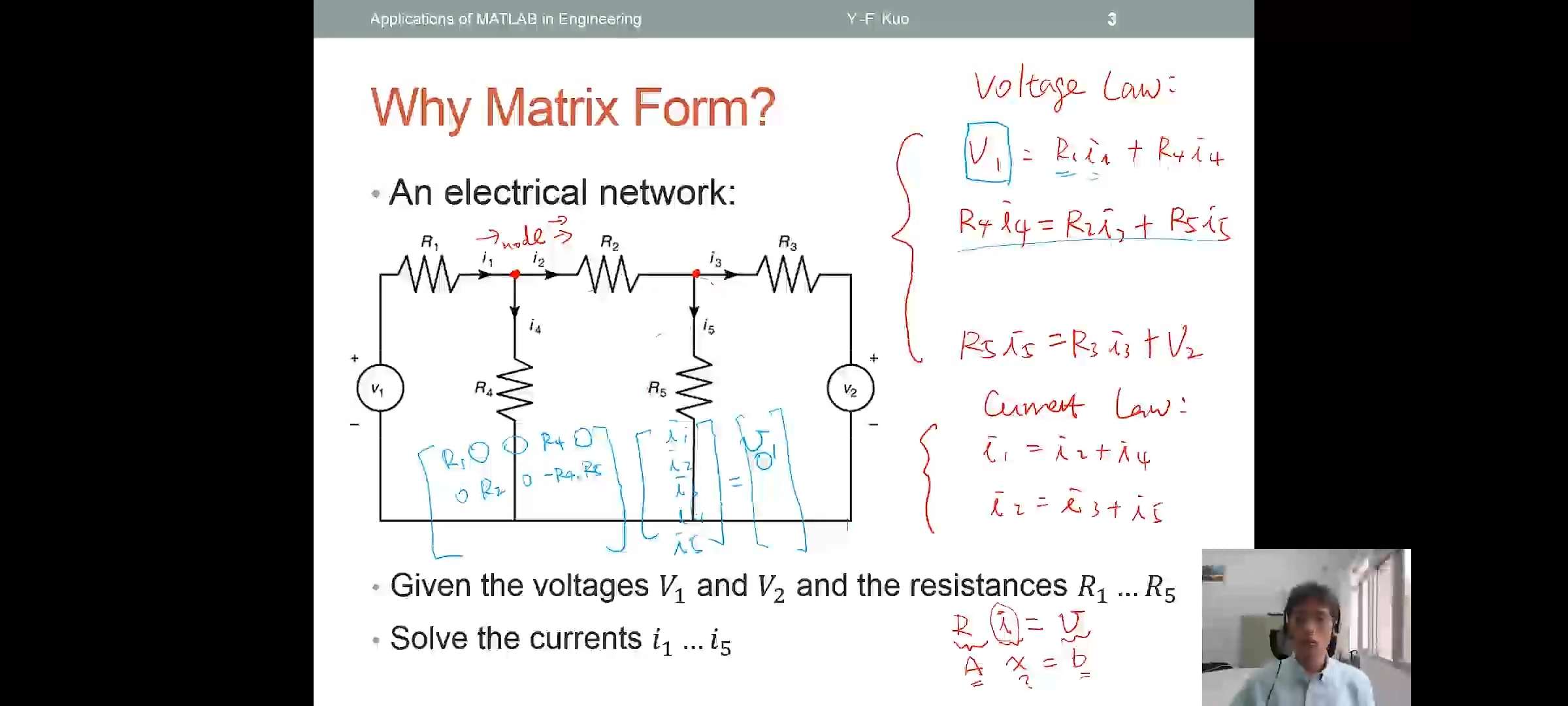
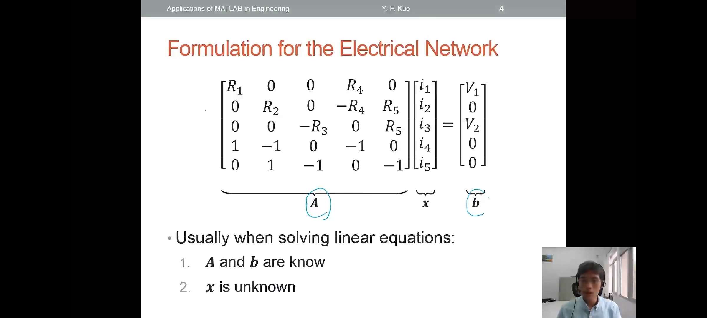
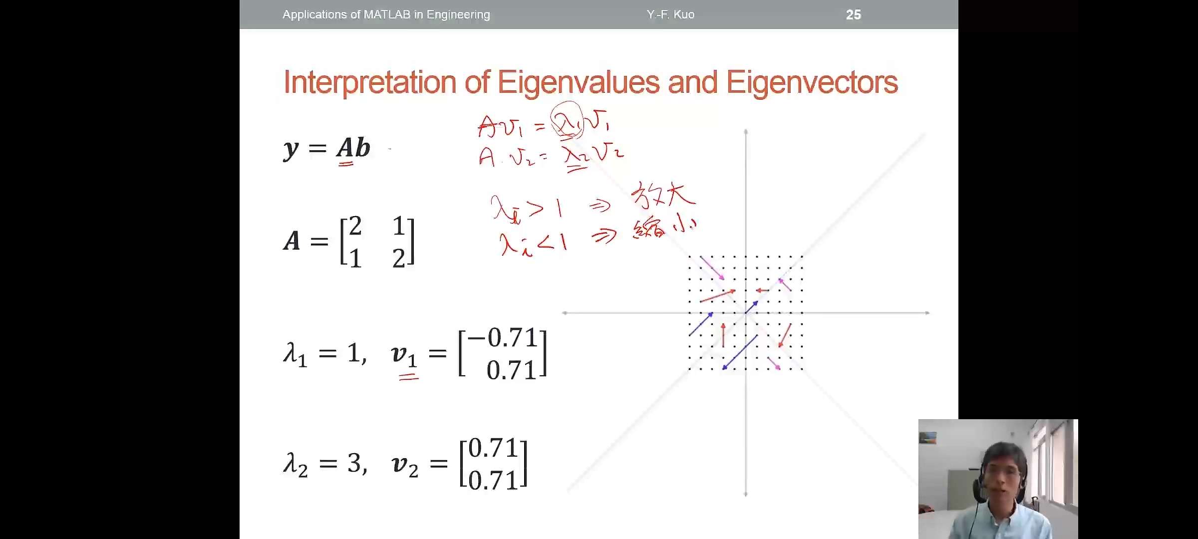
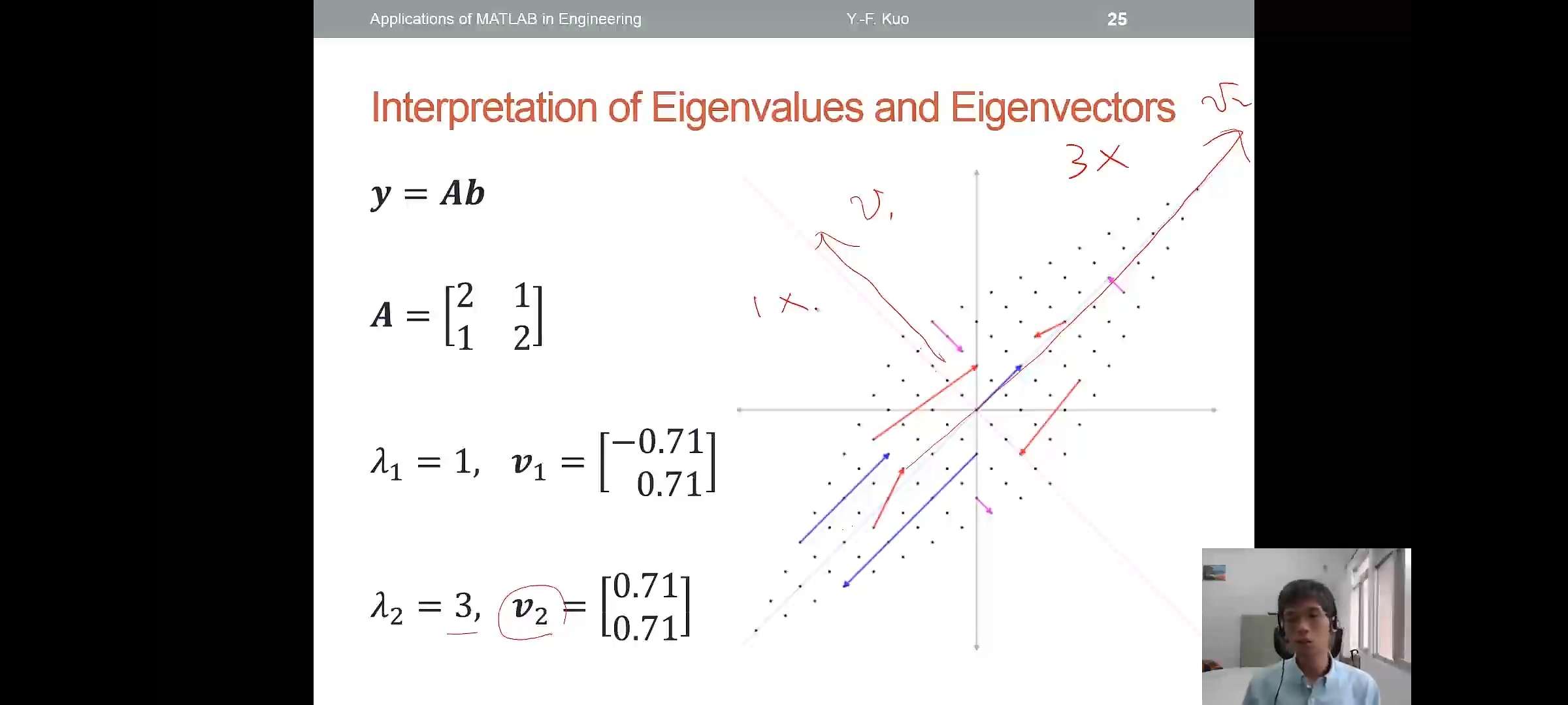
Eigenvalues and Eigenvectors
- For a system \(A \in \mathbb{R}^{m \times
m}\),matrix multiplication \(y=Ab\) is complicated
- Want to find vector(s) \(v_i\in \mathbb{R}^{m \times m}\) such that \[Av_i=\lambda_iv_i\],where\(\lambda_i \in \mathbb{R}^{m \times m}\)
- Then we decompose \(b=\sum
\alpha_iv_i,\alpha_i \in \mathbb{R}^{m \times m}\)
- The multiplication becomes:\[Ab=\sum \alpha_iAv_i=\sum \alpha_i\lambda_iv_i\]
注意上面两张图中右边两个线性系统的变化
Solving Eigenvalues and Eigenvectors
- For given \(Ab=\begin{bmatrix} 2&-12\\ 1&-5\\ \end{bmatrix} \cdot \begin{bmatrix} 2\\ 4\\ \end{bmatrix}\)
\[\lambda_1v_1=-1\begin{bmatrix} 0.97\\ 0.24\\ \end{bmatrix},\lambda_2v_2=-2\begin{bmatrix} 0.95\\ 0.32\\ \end{bmatrix}\]
\[b=\alpha_1v_1+\alpha_2v_2=-41.2v_1+44.3v_2\]
\[Ab=A(\alpha_1v_1+\alpha_2v-2)\\=\alpha_1Av_1+\alpha_2Av_2\\=\alpha_1\lambda_1v_1+\alpha_2\lambda_2v_2\]
eig()
- Find the eigenvalues and
eigenvectors:
[v,d]=eig([2 -12;1 -5])
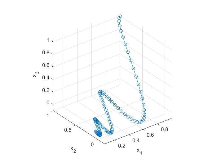
Matrix Exponential:expm()
- A typical linear time-invariant system is usually formulated as \[y=\frac{dx(t)}{dt}=\dot{x}=Ax\]
1 | A=[0 -6 -1;6 2 -16;-5 20 -10]; |
统计
statistics
- The science of "data"
- Involving the collection,analysis interpretation,presentation,and organization of data
- Main Statistical Methodologies
- Descriptive Statistics
- Inferential(推论) Statistics
- Summary Measures
- Central Tendency:Mean(平均数),Median(中位数),Mode
- Quartile(四份位)
- Variation(离散):Range,Variance,Standard Deviation(标准差)
Descriptive Statistics
- Suppose we have samples:
- Variance:\(s=\frac{\sum (x_i-\bar{x})^2}{n-1}\)
- Standard deviation:\(sd=\sqrt{s}\)
- 操作:
| code | 解释 |
|---|---|
mean |
Average or mean value of array |
median |
Median value of array |
mode |
Most frequent values in array |
prctile |
Percentiles of a data set |
max |
Largest elements in array |
min |
Smallest elements in array |
std |
Standard deviation |
var |
Variance |
Exercise:
- Find the following properties of the variable x4
- Mean,median,mode,and quartile
- Range and interquartile range
- Variance and standard deviation
- 加载数据
load stockreturns;以及x4=stocks(:,4);
Figures Are Always More Powerful
- Suppose we have samples:
1
2
3
4
5
6x=1:14;
freqy=[1 0 1 0 4 0 1 0 3 1 0 0 1 1];
subplot(1,3,1);bar(x,freqy);xlim([0 15]);
subplot(1,3,2);area(x,freqy);xlim([0 15]);
subplot(1,3,3);stem(x,freqy);xlim([0 15]);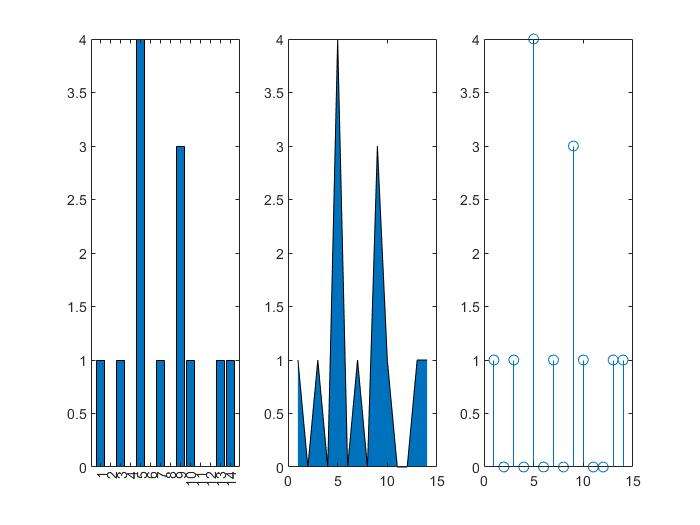
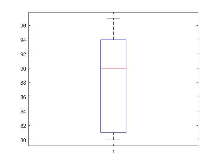
Boxplot
- 描述对象:quartile,median,max,min
1
2
3marks=[80 81 81 84 88 92 92 94 96 97];
boxplot(marks);
prctile(marks,[25 50 75]);
Skewness(扭曲程度)
- A measure of distribution skewness
- Left-skewed:skewness\(\lt 0\),\(Mean \lt Median \lt Mode\)
- Right-skewed:skewness\(\gt 0\),\(Mode \lt Median \lt Mean\)
- Symmetric:\(Mean=Median=Mode\)
skewness()1
2
3
4X=randn([10 3])*3;
X(X(:,1)<0,1)=0;X(X(:,3)>0,3)=0;
boxplot(X,{'Right-skewed','Symmetric','Left-skewed'});
y=skewness(X)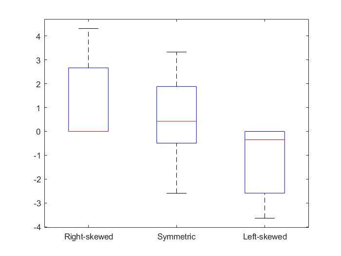
Kurtosis(平缓或尖锐程度)
- A measure of distribution flatness
- A kurtosis of a normal distribution is zero
- Positive Kurtosis:more acute peak
- Negative Kurtosis:more flat peak
Inferential Statistics
- Methods to make estimates,decisions,and predictions using sample data
Statistical Hypothesis Testing
- A method of making decisions using data
- Example:Am I going to get grade A in this class?
- Typical hypothesis:
- \(H_0:\theta=\theta_0\) vs \(H_1:\theta \neq \theta_0\)
- \(H_0:\theta \ge\theta_0\) vs \(H_1:\theta \lt \theta_0\)
- \(H_0:\theta \le\theta_0\) vs \(H_1:\theta \gt \theta_0\)
where \(H_0\) is null hypothesis,and \(H_1\) is alternative hypothesis
Hypothesis Testing Procedure
- Determine a probability ,say 0.95(confidence level),for the hypothesis test
- Find the 95% "confidence Interval" of the \(H_0\)
- Check if your score falls into the interval
- Terminology in Hypothesis Testing
- Confidence interval
- Confidence level\((1-\alpha)\)
- Significance level \(\alpha\)
- p-value
t-test Example
- Are means of the two stock returns(#3and$10) the same?
1
2
3
4
5
6
7
8
9
10
11
12
13
14
15
16load stockreturns;
x1=stocks(:,3);x2=stocks(:,10);
boxplot([x1,x2],{'3','10'});
[h,p]=ttest2(x1,x2)
h =
1
p =
0.0423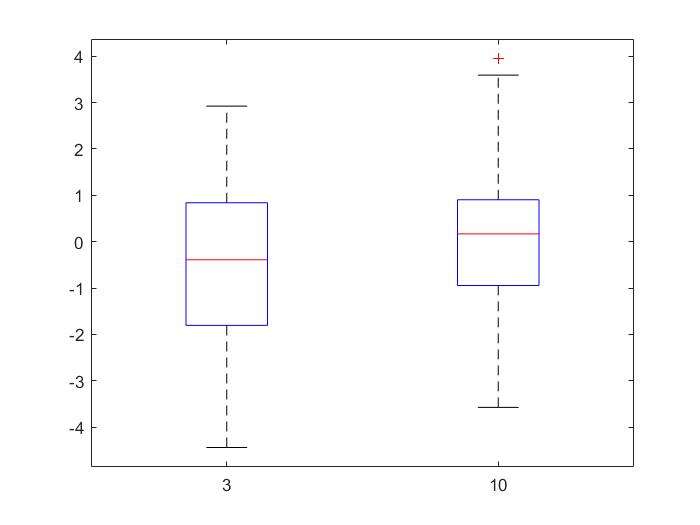
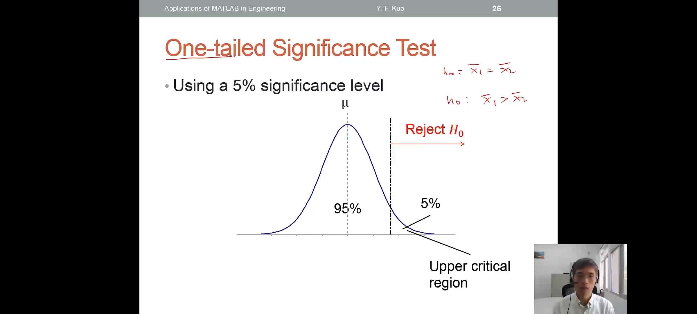
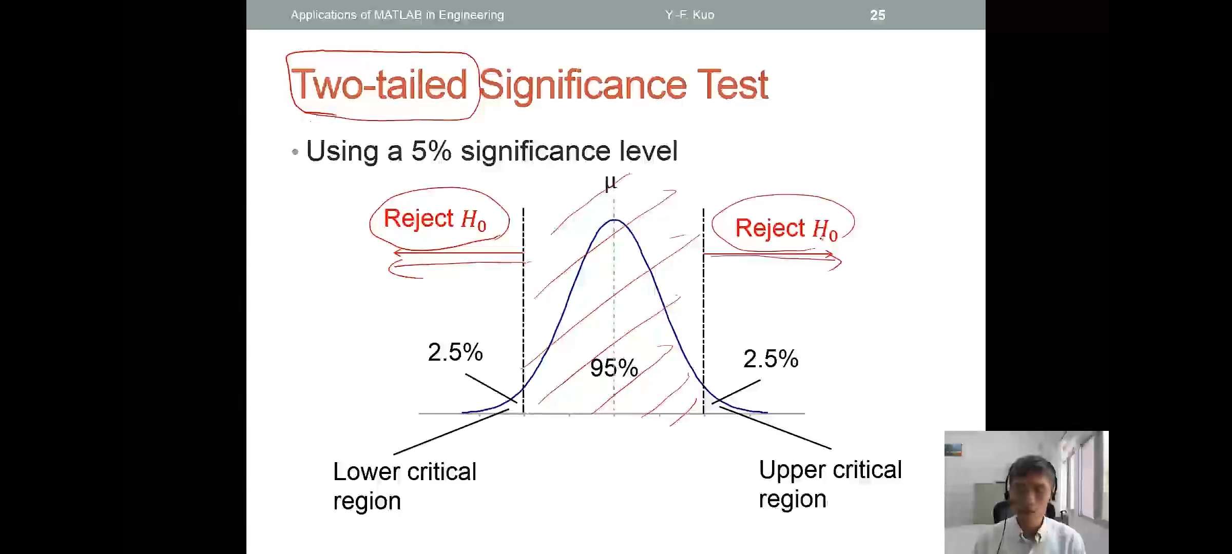
Two-tailed and One-tailed Significance Test
- Using a 5% significance level
Common Hypothesis Tests
| Paired data | Unpaired data | More than two groups | |
|---|---|---|---|
| Parametric | z-test and t-test | two-sample t-test | Analysis of variance (ANOVA) |
| Non-parametric | Sign test and Wilcoxon signed-rank tess | Wilcoxn rank-sum test |
| code | 解释 |
|---|---|
ranksum() |
Wilcoxon rank sum test |
signrank() |
Wilcoxon signed rank test |
ttest() |
One-sample and paired-sample t-test |
ttest2() |
Two-sample t-test |
ztest() |
z-test |
内插与回归
Polynomial curve fitting
Simple Linear Regression
- A branch of data points \((x_i,y_i)\) are collected
- Assume \(x\) and \(y\) are linearly correlated\[\hat{y}=\beta_0+\beta_1x\] \[\epsilon_i=\hat{y}-y\]
Linear Regression Formulation
- Define sum of squared errors(SSE)\[SSE=\sum_i \epsilon_i^2=\sum_i (y_i-\hat{y_i})^2\]
- Given that the regression model:\[SSE=\sum_i (y_i-\beta_0-\beta_1x_i)^2\]
Solving Least-squares Problem
- SSE is minimized when its gradient with respect to each parameter is equal to zero :\[\begin{cases} \frac{\partial \sum_i \epsilon_i^2}{\partial\beta_0}=-2\sum(y_i-\beta_0-\beta_1x_i)=0 \\ \frac{\partial \sum_i \epsilon_i^2}{\partial\beta_1}=-2\sum_i(y_i-\beta_0-\beta_1x_i)x_i=0\\ \end{cases}\]
Least-squares Solution
- Suppose there exists \(N\) data
points: \[\sum_{i=1}^Ny_i=\beta_0N+\beta_1\sum_{i=1}^Nx_i\]
\[\sum_{i=1}^Ny_ix_i=\beta_o\sum_{i=1}^Nx_i+\beta_1\sum_{i=1}^Nx_i^2\]
\[\Rightarrow \begin{bmatrix} \sum y_i\\ \sum y_ix_i\\ \end{bmatrix}=\begin{bmatrix} N& \sum x_i\\ \sum x_i & \sum x_i^2 \\ \end{bmatrix}\cdot\begin{bmatrix} \beta_0\\ \beta_1\\ \end{bmatrix}\]
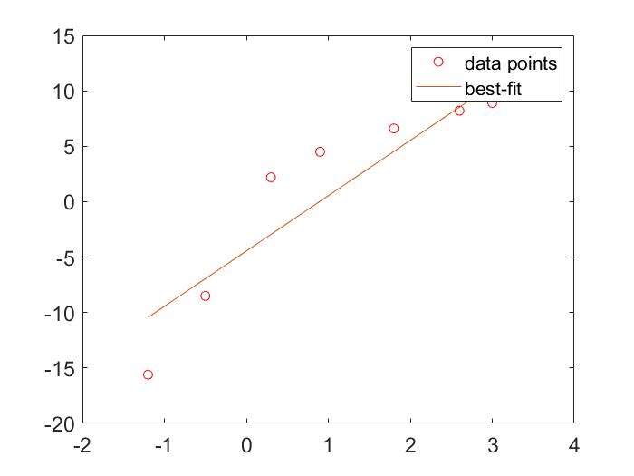
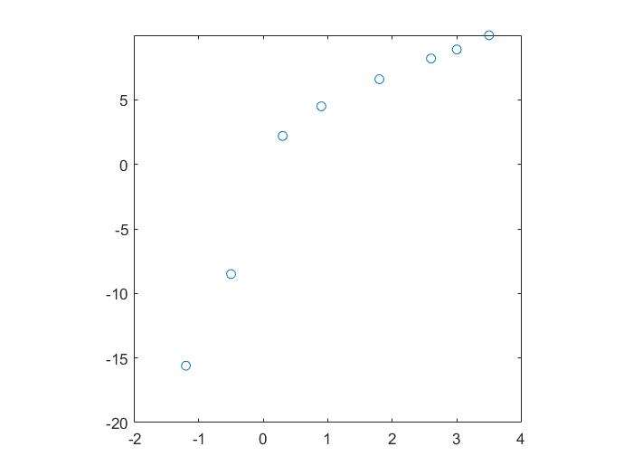
Polynomial Curve Fitting:polyfit()
- Curve fitting for polynomial of different orders
1 | x=[-1.2 -0.5 0.3 0.9 1.8 2.6 3.0 3.5]; |
Eercise:
- Given the table below:
- Find the \(\beta_0\) and \(\beta_1\) of the regression line
- Plot the figure
| TC Output(毫升) | Temperature(摄氏度) |
|---|---|
| 0.025 | 20 |
| 0.035 | 30 |
| 0.050 | 40 |
| 0.060 | 50 |
| 0.080 | 60 |
Are \(x\) and \(y\) Linearly Correlated?
- If not,the line may not well describe their relationship
- Check the linearly by using
scatter():scatterplotcorrcoef():correlation coefficient(相关系数),\(-1 \le r \le 1\)
- 解释:如果得到的图中,点连成的线斜率接近1,则相关性越高。若是-1,则是负相关的
1 | x=[-1.2 -0.5 0.3 0.9 1.8 2.6 3.0 3.5]; |
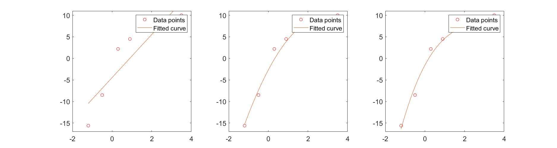
Higher Order Polynomials
Is it better to use higher order polynomials?
1 | x=[-1.2 -0.5 0.3 0.9 1.8 2.6 3.0 3.5]; |
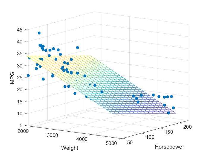
Multiple regression
What If There Exists More Variables?
- Equations associated with more than one explanatory variables:\[ y=\beta_0+\beta_1x_1+\beta_2x_2\]
- Multiple linear regression:
regress() - Note:the function gives you more statistics(e.g.,\(R^2\))of the regression model
Ex:
1 | load carsmall; |
What If the Equations Are NOT Linear?
- What are linear equations?
- \(y=\beta_0+\beta_1x_1+\cdots+\beta_nx^n+\beta_mx_1x_2\)等形似方程是linear
DC Motor System Identification
For a typical DC motor,the celocity \(v(t)\) and displacement \(s(t)\) pofiles of a step reponses of are
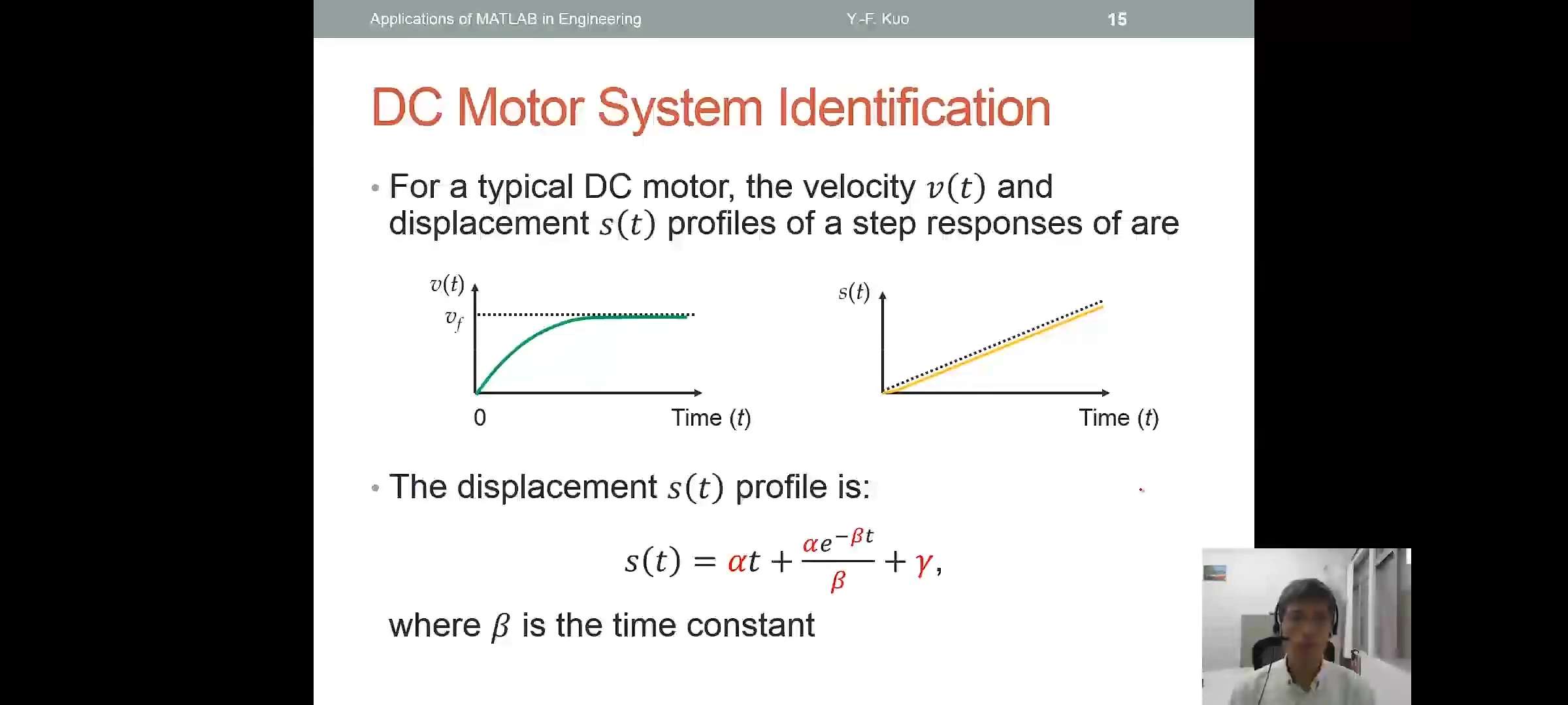
The displacement \(s(t)\) profile is:\[s(t)=\alpha t+\frac{\alpha e^{-\beta t}}{\beta}+\gamma\]
where \(\beta\) is the time constant
Cure Fitting Toolbox:cftool()
Interpolation(插值)
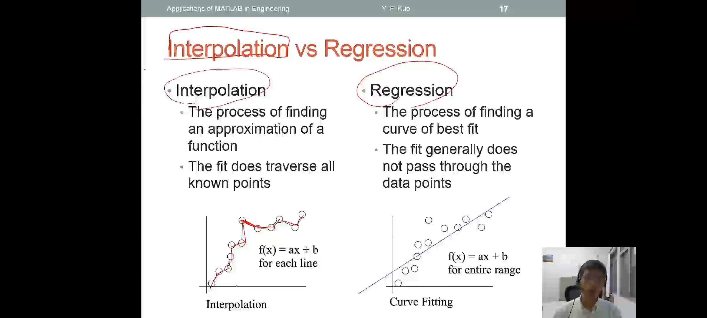
- Interpolation
- The process of finding an approximation of a function
- The fit does traverse all known points
- Regression
- The process of finding a curve of best fit
- The fit generally does not pass through the data points
Common Interpolation Approaches
- Piecewise linear interpolation
- Piecewise cubic polynomial interpolation
- Cubic spline interpolation
| code | 解释 |
|---|---|
interp1() |
1-D data interpolation (table lookup) |
pchip() |
Piecewise Cubic Hermite Interpolating Polynomial |
spline() |
Cubic spline data interpolation |
mkpp() |
Make piecewise polynomial |
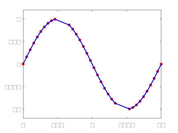
Linear Interpolation:interp1()
1 | x=linspace(0,2*pi,40); x_m=x; |
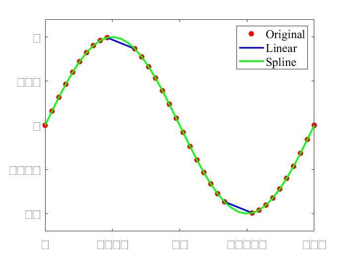
Spline Interpolation:spline()
1 | %接着上面的程序 |
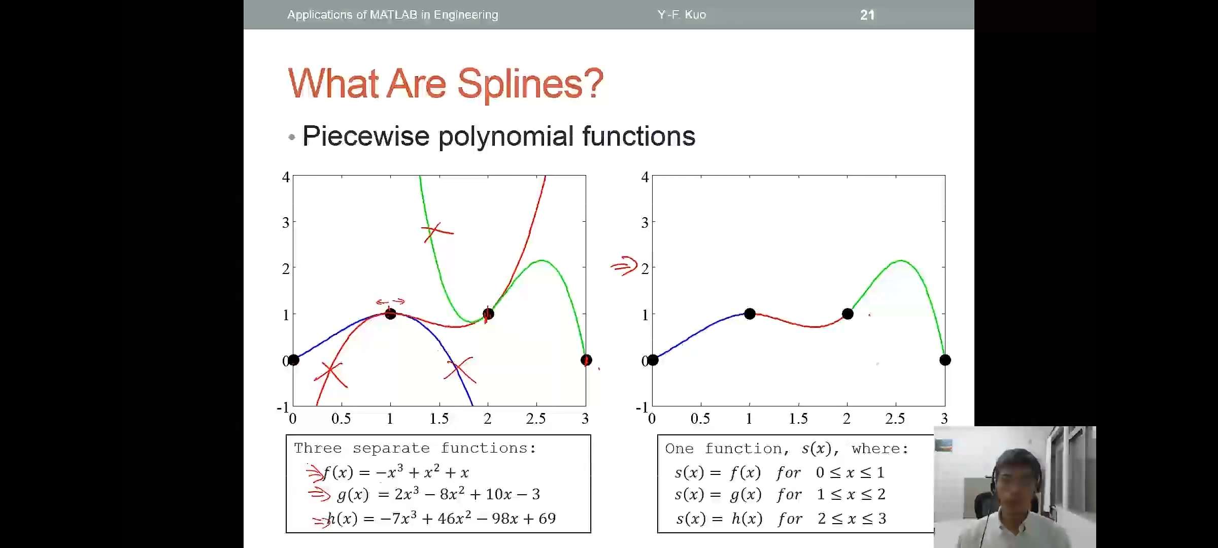
What Are Splines?
- Piecewise polynomial functions
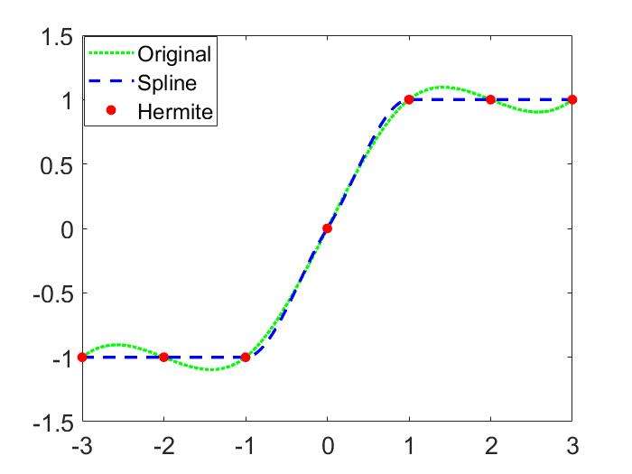
Cubic Spline vs Hermite Polynomial
1 | x=-3:3; y=[-1 -1 -1 0 1 1 1]; t=-3:.01:3; |
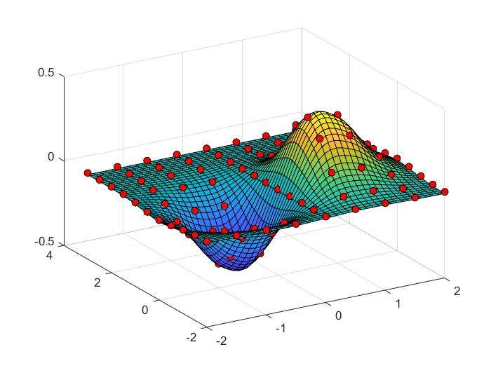
2D Interpolation:interp2()
1 | xx=-2:.5:2;yy=-2:.5:3; |
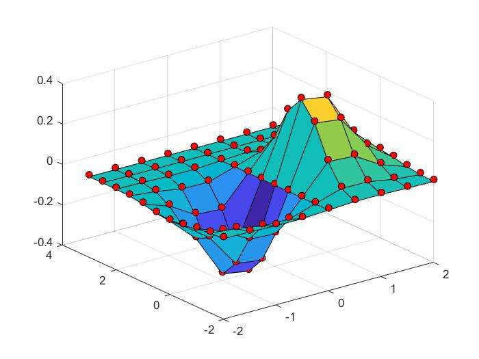
1 | %接着上面的程序 |
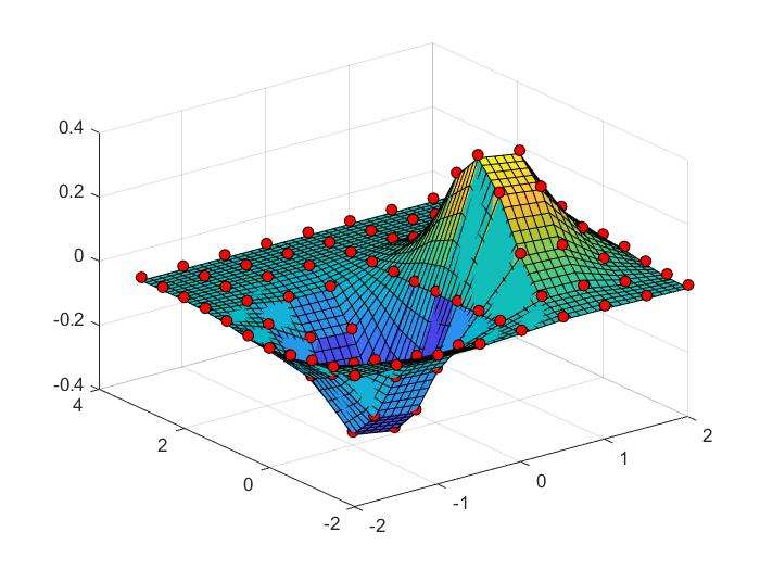
2D Interpolation Using Spline
1 | xx=-2:.5:2;yy=-2:.5:3; |